- through the creation of a k-nearest neighbor graph (k-NNG), followed by graph layout and clustering algorithms
- through dimensionality reduction (DR) and non-graph based clustering algorithms
TL;DR
Dimensionality reduction using UMAP is the faster and more precise method, and should be preferred unless the focus is on analysis of longish natural language texts. In the latter case, the k-NNG method currently provides a measure of text similarity that usually works a little better. Also, if the dataset contains a broad mix of quantitative and categorical variables, and UMAP dimensionality reduction does not generate the desired result, k-NNG may be worth trying, as it sometimes achieves a better balance between columns of different type.K-nearest neighbor graph
Overview
The k-NNG approach (k-Nearest Neighbor Graph) constructs a graph (network) where each point in a dataset is connected to the k other points most similar to it. On its own, this simply constructs an abstract graph, consisting of nodes that represent the rows in the dataset, and links connecting them if they are similar enough. In order to be able to view this graph on the (2-dimensional) screen, the nodes need to be assigned coordinates in the x/y plane. This is usually referred to as calculating a layout for the graph. The method employed in Graphext to do this is a force-based layout, which aims to place points such that the length of links reflects the similarity between them, while also aiming to avoid links crossing each other. We have chosen the forceAtlas2 layout algorithm as a sensible default, as it tends to work well enough across a variety of use cases. The resulting graph, laid out on the 2-dimensional screen, can be thought of as an “embedding”. We have effectively embedded the original dataset in the space of x/y coordinates such that the positions of nodes reflect the similarity or dissimilarity between their corresponding dataset rows. While certain structures, like clusters of related points, are often immediately visible to the naked eye in such graphs, their identification can further be automated using clustering algorithms (in the context of graphs/networks also referred to as community detection). In Graphext, we use the Louvain algorithm as a sensible default to detect clusters in graphs, as it produces good results in most cases. It also has the advantage of being fast to calculate, and so we can offer to re-calculate it on-the-fly from within Graphext’s UI (using the “Automatic segmentation” feature).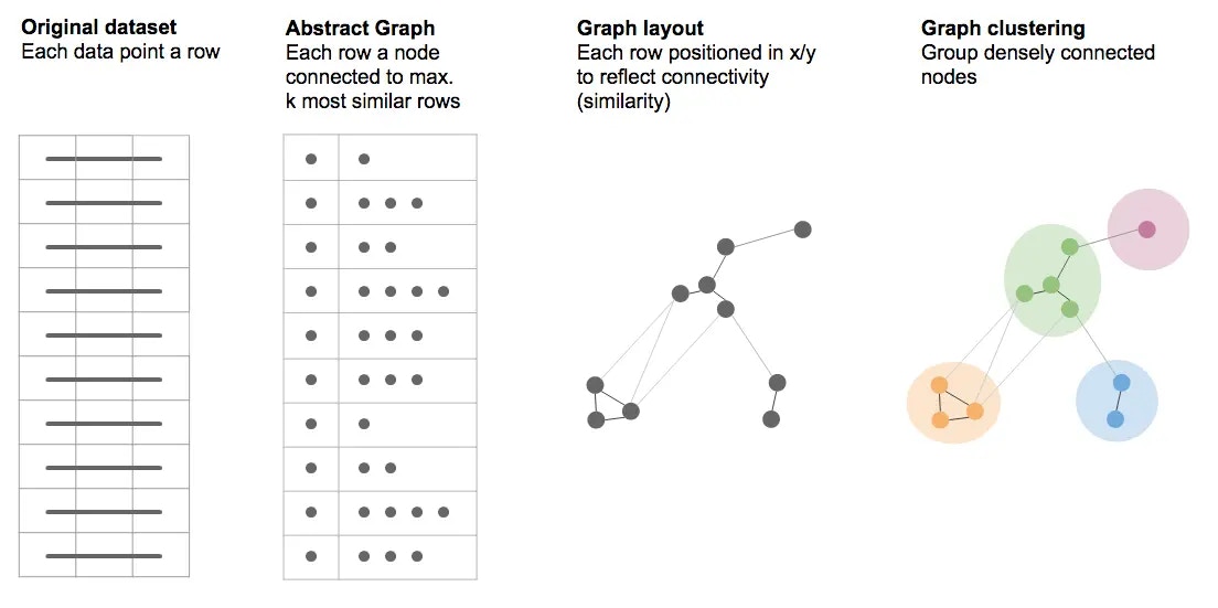
Figure 1: k-NNG flowchart. First, each row is associated with no more than the k most similar rows in the dataset, creating a (still abstract) graph. A layout is then calculated that positions the graph nodes in two dimensions (x/y) such that similar, connected rows are positioned close to each other. In a last step, the graph is clustered such that closely related groups of rows can be more easily identified.
Technical details
Constructing the k-NN graph
Construction of a k-NN graph is simple if one is able to measure the similarity between pairs of data points. E.g. if a dataset only contains numeric columns, and each data point is thus a simple list of numbers (vector), we can simply use the Euclidean distance to measure the similarity between two points (the straight-line distance between points in what we intuitively consider the normal 2d, 3d, or n-dimensional space, such as the x/y plane we know from school). This approach is not applicable, however, if the dataset contains other types of data, such as categorical columns, dates, free-form natural language text and so on, since now we cannot easily interpret points as living in such a simple space (e.g. what would we be the coordinates of a categorical variable?). This means we need another measure of similarity that can be applied to datasets having mixed types of data. In Graphext, our choice is a custom measure that is somewhat similar to what’s known as the Gower distance. The idea is simple: to measure the similarity between two data points, we apply a different measure for each type of column. E.g., for each numerical column we may apply some form of normalized difference between the quantitative values; for categorical columns we may simply check if the two points belong to the same category (distance = 0) or not (distance = 1); for text columns we may calculate similarity in terms of common word usage, etc. The final similarity then is simply the weighted average of all these individual column-wise measures. Since this provides a way to compare two points with arbitrary data types, we can then simply calculate the distances between all pairs, and use these to generate the k-NN graph.Graph layout with forceAtlas2
We use our own (fast, C++) implementation of the force-based layout algorithm forceAtlas2. The basic idea of this algorithm is that nodes generally repel each other, while links act as springs applying an attracting force between connected nodes. The algorithm applies these forces to the nodes iteratively until a stable configuration is found in which the forces all balance out and the nodes stop moving (mostly). If the result is not ideal for a given dataset, e.g. nodes being too close together, or too far apart, the algorithm has a number of parameters that can be changed to create aesthetically different results (never changing the actual connectivity, and so also having no influence whatsoever on any clustering applied to the network, for example).Graph clustering with Louvain
For graph clustering we also have our own, optimized implementation of the Louvain algorithm (written in Rust, and compiled to also work in the browser, i.e. from the Graphext UI). Louvain iteratively assigns nodes to clusters such as to maximize a measure called modularity, which is the relative density of edges within clusters with respect to edges between clusters. In other words, it tries to assign nodes to clusters such that there are many more connections between the nodes in the same cluster than there are between nodes in different clusters. As with the forceAtlas2 layout, the default configuration should generate decent results in most cases. However, a somewhat common occurrence is the generation of either too many or too few clusters. This can easily be addressed, however, as the algorithm has a resolution parameter that influences the number of clusters generated. For further details see the documentation of the corresponding cluster_network step.Advantages & disadvantages
Advantages
- Works without having to preprocess mixed-type data, as we can use a different metric for each data type. This means less uncertainty about how the data is treated before any other algorithm is applied.
- Currently has the better metric for comparing longer texts (based on Tf-Idf, rather than word embeddings as used in the dimensionality reduction method explained below). Though this may change in the near future.
Disadvantages
- High complexity, i.e. slow execution time. The algorithm does not scale well, as the size of the dataset grows. Since we need to calculate the similarities between , the execution time scales quadratically with the number of rows. A dataset with twice the number of rows will take 4 times longer to process. More precisely, the complexity of the approach for d input dimensions and n rows scales as O(d * n^2).
- Doesn’t always work well with unusually distributed data (non-normal). For example, if a numerical column has a bi-modal distribution, i.e. with points being separated into two (or more) disparate regions, than (dis)similarity will be over-emphasized if two points fall into different regions, while similarity will be de-emphasized if two points fall within the same region. Effectively this means a loss of precision within each of the disparate regions, which in turn may result in a failure to separate some clusters.
When to use
Since it doesn’t scale very well for larger datasets, we recommend the k-NNG method principally for analyses with a focus on longish natural language text, where the current Tf-Idf similarity tends to provide slightly better results than the word embeddings used in the dimensionality reduction approach. Also, if the dataset contains a broad mix of quantitative and categorical columns, and dimensionality reduction does not provide the desired result, it may be worth trying with k-NNG, as sometimes it achieves a better balance between columns of different data types.How to use in Graphext
Creating a k-NN graph in recipes
For each step in the k-NNG as described above, there is a corresponding method in Graphext to be used in recipes. A partial recipe may look like this, for example:link_similar_rows creates the abstract graph. Given an input dataset, the step’s output is a new dataset (links) in which each row is a link connecting one row to another. It has 3 columns: source, target and weight. The first two refer to the ids of the rows that are connected by the link (row numbers), while the weight column contains the numerical value of the similarity between the two rows.
To calculate node x/y positions we use the step layout_network. This takes the just generated links dataset, and adds the x and y columns to the original rows, such that each row/node now has an associated position.
Finally, we detect clusters in the graph with cluster_network. This step also receives the links dataset as input, and returns a simple categorical column containing the cluster labels.
Creating a k-NN graph using the Wizard
Details may vary depending on the version of Graphext (if used on-premise), and the particular choice of analysis selected initially in the Wizard, such as whether you’ve chosen to do a specific analysis of customers, say, or a generic segmentation (Other); but in most cases you should be able to select the option of doing a simple Segmentation (or Segment your data), which without further qualification means a clustering using the k-NNG approach (selecting Segmentation using UMAP & HDBSCAN, on the other hand, would correspond to the dimensionality reduction approach). In newer versions of the Wizard, you may also find a Network and Clusters panel in the Advanced Settings section. Here you should be able to select k-NNG & Louvain as the Dimensionality reduction and clustering algorithms option. This will automatically configure the recipe to include the steps as shown above (or similar).Frequently asked questions
Why does the k-NNG approach not separate some of my cluster, when I think they should be separable?
- One reason may be that the data in the two supposed groups is really not different enough for any similarity metric to tell the difference.
- Another reason may be the loss of precision of this method with non-normal data, as mentioned in the Disadvantages section above. Check if any of your variables have a bi-modal distribution (with two distinct peaks instead of one), for example. If this is the case, you may want to try the dimensionality reduction approach instead.
- You may also find large undifferentiated “hairball” networks if the number of neighbors used to create the network is too large when compared to the size of the dataset. If you have a small dataset (say 100 rows), and you connect each row to a large number (say 20) of other rows, you may find that “everything becomes connected to everything”, and so there is no structure in the graph for the layout and clustering algorithms to work with. In this case try reducing the
n_similar_docsparameter inlink_similar_rows.
My recipe seems to take a long time, how do I make it go faster?
As mentioned, the k-NNG approach is inherently slower than the dimensionality reduction described in the next section. The only way to reduce execution time somewhat is to use fewer variables, i.e. passing a smaller subset of columns to thelink_similar_rows step.
Dimensionality reduction
Overview
Dimensionality reduction as layout
Our second approach to embedding data points is based on dimensionality reduction, and more specifically (at least for now), the UMAP algorithm. The idea, in this case, is to find a new way to represent our data using a smallish number of numerical columns (e.g. x and y only), but such that distances measured on our dimensionally reduced dataset maintain the same neighborhood structure as the original data. In other words, we want to find x/y positions for each data point, such that rows in the original dataset that are very similar will be found close to each other in terms of their x/y positions; and rows that are very dissimilar in the original dataset should be farther away from each other in terms of x and y. UMAP is a mathematically sound and principled approach to do just . Thus, when using dimensionality reduction (whether UMAP or other algorithms), we do not explicitly create a graph of nearest neighbors, and then calculate a layout. We rather consider the dimensionally reduced dataset itself our layout. Or, to state the same in reverse, to layout our dataset, we directly reduce our dataset to two dimensions (using UMAP or other algorithms) and interpret these as the data points’ x and y positions.Dimensionality reduction for clustering
Note that the fewer dimensions we retain, the more information . When calculating the 2-dimensional layout, the goal therefore is to at least capture the most salient structures in the dataset (e.g. clusters, the relative similarity between different clusters, local differences within clusters etc.). However, we do not have to restrict ourselves to always reducing our data to two dimensions only. For any purpose other than visualizing the dataset on the screen, it may make sense to keep more than two dimensions (and therefore more of the original information). This applies e.g. when trying to identify clusters. It may be, for example, that certain clusters can only be separated well in 3 dimensions (as an analogy, imagine e.g. one cloud behind another, and being able to distinguish them only from certain angles). In graphext, we therefore often embed our dataset twice using dimensionality reduction:- Once, with exactly 2 dimensions for visualizing the dataset
- A second time, with about 10 dimensions for the purpose of clustering
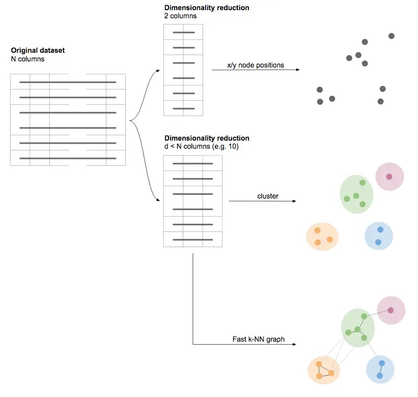
Figure 2: Dimensionality reduction flow-chart. A dataset is reduced first to two dimensions to generate a layout (x/y positions). It is then reduced a second time to ~10 dimensions. This latter dataset is then used to calculate a clustering (using e.g. HDBSCAN), as well as to identify each row’s nearest neighbors, which allows linking the laid out nodes into a connected graph.
Technical details
Preprocessing for UMAP
The vast majority of machine learning algorithms, including dimensionality reduction techniques like UMAP and cluster algorithms such as HDBSCAN, require their input data to be purely numerical and without any missing data. Few algorithms provide support for other data types (such as categorical, date and time etc.), for a mix of different types in the same dataset, or support missing data out of the box. Graphext therefore provides a way to convert a dataset with arbitrary data types into a purely numerical dataset without missing data. It does so by defining for each possible type of input column a transformation from non-numeric to numeric values. As an example, ordered categorical variables (ordinals) such as the day of week, may be converted into a series of numbers (0..7). Non-ordered categorical variables of low-cardinality (containing few different categories) may be expanded into multiple new columns of 0s and 1s, indicating whether each row belongs to a specific category or not (one-hot encoding). Similar transformations are applied to dates, multivalued categoricals etc. Missing values (NaNs) are imputed, i.e. replaced with an appropriate value from the corresponding column (e.g. the median in a quantitative column). In addition, a new column of 0s and 1s is added, indicating whether the original column had a missing value or not. All this is done automatically behind the scenes whenever you pass a dataset to an algorithm that expects its input to be numerical and complete. While this is convenient (since otherwise essentially no machine learning algorithm would be applicable to real-world datasets), it is currently not configurable, and so in specific, and hopefully rare, cases the way missing data is handled may not be ideal, for example. Note, however, that most of the time the machine learning algorithms we apply to your data are not supposed to give you the most precise predictions possible. Rather, the goal is to help you more easily explore your dataset and generate hypotheses (which you may then want to confirm or not using a more targeted approach).Clustering using HDBSCAN
For many clustering algorithms it is difficult to determine in an intuitive way how many clusters should be found. In k-means, for example, you need to know beforehand how many clusters you’d like to identify, while many times such information is not available a priori. Other algorithms (such as Louvain, described above), may provide a resolution parameter, but again, it is not usually obvious how to select it. HDBSCAN tries to address this problem with a more intuitive configuration. Its main parameter influencing the resulting number of clusters is min_cluster_size, which as the name implies, is the minimum number of data points any group should have to be considered a cluster. Intuitively, HDBSCAN will (hierarchically) identify clusters of densely packed points, where groups smaller than min_cluster_size are considered noise if not part of a larger cluster in the hierarchy.Adding explicit graph and Louvain clusters for UX consistency
As described above, although no explicit nearest neighbour graph is needed in principle to use the dimensionality reduction approach (neither for creating a layout, nor for clustering), Graphext will usually derive one anyway from the dimensionally reduced embeddings. Having the connectivity between data points available allows for easier navigation between neighbours in the UI, for example, and allows for the use of Louvain to cluster all or parts of the dataset on the fly (“automatic segmentation”). Note that the step to create this connectivity is not the same as the k-NNG approach however. Since we already have our dimensionally reduced embeddings (e.g. as the output of the embed_dataset step), we can use very fast algorithms to find each row’s nearest neighbour (we use Spotify’s Annoy here), and so this extra step does not add significant computational overhead.Advantages & disadvantages
Advantages
- Unlike the k-NNG approach, it doesn’t make any assumptions about the distributions of input variables. It therefore also doesn’t suffer from a loss of “precision” in the case of non-normal data.
- It scales better with increasing number of rows. Behind the scenes, the algorithm doesn’t need to calculate all pairwise similarities, but uses an approximation instead to find nearest neighbors. This means it doesn’t scale quadratically (the approximate complexity seems to be around O(d*n^1.14) for d input dimensions and n rows, also see here).
- It is a published algorithm with strong mathematical justification and proven usage in various fields (single cell analysis, neural network activations, time series analysis and more).
Disadvantages
- As explained in Technical Details, the UMAP approach relies on inputs being numerical, which means we need to first transform any non-numerical data before applying the algorithm. Since this is done behind the scenes (for simplicity on the user side), and currently not configurable, this leads to less transparency in what data is eventually processed during dimensionality reduction and clustering.
- To be able to provide dataset “navigability” in Graphext, i.e. being able to select a node’s neighbors etc., an explicit k-NN graph is eventually constructed anyways, although not in principle necessary for neither dimensionality reduction nor clustering. Though fast in terms of execution, this leads to somewhat more complexity in recipes using this approach (also see Fig. 2).
When to use
Ignoring recipes provided out-of-the box in Graphext, we recommend using the dimensionality reduction approach with UMAP as default in most cases, more so when datasets are large, or when little is known about the distributions in the data. UMAP is considerably faster, and generally more precise in maintaining both local and global similarity between data points. When analyzing longish texts, however, the text similarity measure used by the k-NNG approach works a little better sometimes. Also, when working with a lot of mixed variables types (numerical, categorical etc.), the k-NNG may be worth trying, since in some cases it seems to achieve a better balance between the different types.How to use in Graphext
Performing a dimensionality reduction in recipes
Again, each step in the flowchart for dimensionality reduction corresponds to a step/method in Graphext recipes. For example:layout_network is used to reduce the input dataset to 2 dimensions (x/y) using UMAP. Next, embed_dataset employs UMAP again to create 10-dimensional embeddings. In the resulting output column, each original dataset row is now represented by a .
Having embedded the dataset in 10 dimensions, we then use cluster_embeddings with the HDBSCAN algorithm by default to identify clusters in the dataset. Finally, link_embeddings is used to calculate for each embedded row its k nearest neighbours. The output is again a dataset of links indicating which nodes should be connected as well as how similar they are quantitatively.
Performing a dimensionality reduction using the Wizard
Again, details may vary depending on the version of Graphext (if used on-premise), and the particular choice of analysis selected initially in the Wizard; but if the type of analysis supports the use of dimensionality reduction, then you should be able to select something like Segmentation using UMAP & HDBSCAN as an option from the first set of questions (if the segmentation option doesn’t specify any concrete method, the k-NNG approach is used instead). In newer versions of Graphext, you may also find a Network and Clusters panel in the Advanced Settings section of the Wizard. Here you should be able to select UMAP & HDBSCAN as the Dimensionality reduction and clustering algorithms option. This will automatically configure the recipe to include the steps as shown above (or similar).Frequently asked questions
UMAP (embed_dataset) is still taking a long time, how can I accelerate its execution?
Although UMAP is already pretty fast (when compare to related algorithms like t-SNE), for very large dataset there are a number of tweaks that increase performance at the cost of a possible (but not necessary) reduction in precision:- random_state: if determinism is not required, the parameter
random_statecan be set to null ({“random_state”: null}). This will enable parallel execution of the UMAP algorithm. This is still an experimental feature and so may or may not result in faster performance. It will, mean, however, that repeated executions of the step, even with identical input data, may produce different results. Note that these differences are usually negligible, i.e. they will not change any of the general structures inherent in the data, and therefore won’t usually affect any insights that can be derived from it. - init: by default, before applying its own logic to the data, UMAP initializes the layout of data points using the “spectral” method. For large dataset this can be somewhat costly. In this case you may also try with
{“init”: null}, which should be faster, at the cost of potentially being less precise. - n_neighbors: this parameter controls how many nearest neighbors UMAP takes into account when calculating the layout/embedding. The smaller the number, the faster the execution and the greater the focus on the local structure of the data. The greater the number, the slower the execution and the greater the focus on the larger-scale structures in the data.
Some clusters seem very far apart. How can I avoid large distances between clusters?
In some cases, if clusters are sufficiently different from each other (if the corresponding graph is essentially disconnected), UMAP may push the clusters rather far apart from each other. Visually this means individual points may become small in the UI, and although this doesn’t affect the “quality” of the embedding, it may make navigating the resulting layout less convenient. In this case you may try to change the parametern_epochs (which is 200 by default for large datasets and 500 for smaller ones). Setting this to smaller values means the algorithm will have less time to push clusters apart, but also less time to converge on the “optimal” solution.
I see strange long threads of data points in the UMAP layout, instead of more patch-like clusters. What happened?
This is usually a sign that you’ve used only (or principally) input columns that are (nearly) unique, i.e. have a different value in each row. Typical cases are e.g. the use of numeric customer IDs or dates, where each row has a different ID or date. If this is the only information the algorithm has to go on, then each row will essentially be connected to the next higher and lower ID or date, and the result will be a more or less tangled thread of data points with values increasing or decreasing from one end of the thread to the other. Simply include more informative features in the corresponding steps to create a proper clustering.But does it work?
Since the embedding of a dataset, and its clustering, is usually done unsupervised, i.e. without knowing the ground truth for at least part of the data, there is no direct way to confirm whether a particular clustering is “correct”, or even any “good” or “bad”. In fact, without a ground truth, or some other context, any clustering whatsoever is as valid as any other. What matters in this case, usually, is whether the clustering is useful. Being useful here could mean, e.g., that different clusters of customers correspond to my intuition about the groups of customers I expect; or that the clusters allow me to predict, understand or classify customer behaviour more easily when compared to not distinguishing between groups of them.Validation with labelled data
Fortunately, for the purpose of evaluating a particular approach or algorithm, we can make use of labelled data (where the ground truth is known) to get an idea of its usefulness. The idea here is simply to see whether the clusters identified automatically and from the features of the dataset alone, correspond to the labels a human has assigned to data points manually. E.g., the famous Iris dataset, contains information about 3 different species of Iris flowers. It provides 4 variables that describe the shape of their petals and stalks, as well as a 5th column indicating the species (versicolor, setosa or virginica). To see whether any of Graphext’s embedding and clustering approach actually “works”, we simply embed and cluster the dataset using the four feature variables only, and then compare whether the found clusters of flowers correspond to the different species as identified in the label column. In other words, we’d expect all flowers in the same, automatically identified, cluster to be of the same species, even though we haven’t used information about species in the clustering. Of course, this will only work if the features provided in the dataset correlate to a sufficient degree with the labels. If the measured features of the flowers didn’t tell us anything about their species, then a clustering wouldn’t be able to “recover” the species either. Fortunately, there are many datasets used to benchmark classification algorithms, which we can simply re-purpose for the task of cluster evaluation. Doing this for a sufficiently diverse number of datasets (in terms of size, complexity, data types etc.), we can convince ourselves that, and to which degree, each approach recovers the original labels. We include and share a number of projects doing just this in the Graphext team Validation (you may need to ask us to add you to the team to be able to access it). All projects here are based on typical datasets used to benchmark classification algorithms. As such, each contains the human-annotated ground-truth labels in a categorical column, which we’ve pinned to the top of the left column in the Graphext UI. Just below on the left, you’ll then find the clusters we’ve identified without taking into account the true labels. To easily compare the two, you can e.g. color the nodes by the true labels and confirm that each true class corresponds to one (or more) clusters (sometimes automatic clusters will make a finer or coarser distinction between groups of similar data points). E.g., in the Iris project, with color and node title indicating the true species, the following figure confirms that automatic clusters almost perfectly distinguish the 3 different species: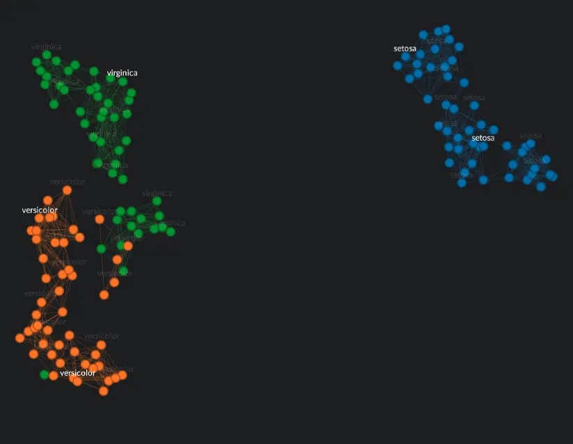
Figure 3: The Iris dataset laid out with UMAP and nodes colored using the true label (species). One can see easily that almost all nodes of the same species fall into a particular region/cluster. The few nodes that get mixed up with other species correspond to exactly those examples of their species having unusual characteristics that make them appear similar to another.
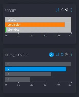
Figure 4: Selected HDBSCAN clusters in the Iris project, and the number of nodes belonging to each species. Cluster 0 has only nodes of the “setosa” species, while cluster 2 almost only contains nodes with the “versicolor” label.
Example validation projects
We have included a variety of different datasets and projects in the Validation team. For each dataset we have created at least one project using the UMAP approach, and one using the k-NNG approach, with the name indicating which was used. The ground truth labels are always to be found on the top-left, followed by the automatic clusters. See the box below for a list of current validation projects (at the time of writing).Example projects
Example projects
- Iris (Scikit-learn dataset) 150 rows, 4 numeric features. Classes: 3 species of flowers.
- Penguins (Dataset on github) 344 rows, uses the 4 numeric features. Classes: 3 species of penguins.
- Wine (Scikit-learn dataset) 178 rows, 13 numeric features. Classes: 3 types of wine.
- Breast cancer (Scikit-learn dataset) 569 rows, 30 numeric features. Classes: 2 (malign, benign)
- Mushrooms (UCI dataset) 8124 rows, 21 categorical features, 1 numerical. Classes: 2 (edible, poisonous)
- Adults (UCI dataset) 48,842 rows, 6 numeric features, 9 categorical. Classes: 2 incomes (<= 50k, >50k)
- Nist Digits (Scikit-learn dataset) 5,620 handwritten digits, each image containing 8x8=64 pixels. 10 classes (0, 1, …, 9).
- Fashion Mnist (Dataset on Github) 70,000 images of clothing items, 28x28 pixels. Classes: 10.
- News (Scikit-learn dataset) 18,846 newsgroup posts (message body only). Classes: 20 (newsgroup topics).
Summary
We have given an overview of the two principal approaches to laying out a dataset in Graphext:- Building a k-nearest neighbor graph and applying graph-based clustering (Louvain). The recipe steps involved here are link_similar_rows, layout_network, and cluster_network.
- Using dimensionality reduction (UMAP) and density-based clustering (HDBSCAN). The recipes steps involved here are primarily layout_dataset, embed_dataset, and cluster_embeddings.