> ## Documentation Index
> Fetch the complete documentation index at: https://docs.graphext.com/llms.txt
> Use this file to discover all available pages before exploring further.
# Graphs and data types
## Introduction
[*UMAP*](/guides/graphs/#dimensionality-reduction-as-layout) and our proprietary [*k-NN*](http://127.0.0.1:8000/guides/graphs/#overview) graph treat the relative balance between categorical and numeric data differently, leading most of the time to qualitatively different embeddings. The k-NNG method has a tendency to clearly separate the network into clusters such that each cluster corresponds to a combination of categories (across different variables). UMAP tends to not divide the network as sharply based on categorical columns, yet can be configured to give them more or less influence on the resulting embedding.
## Example 1 – Human resources data
As a first example, we use a human resources dataset with 10 numeric and 2 categorical columns. The categorical columns represent the *salary* of employees (3 levels) and their *department* (10 levels). We will also be showing two numeric columns: the *number of projects* (integer values from 2 to 7), and *satisfaction level* (continuous in \[0, 1]).
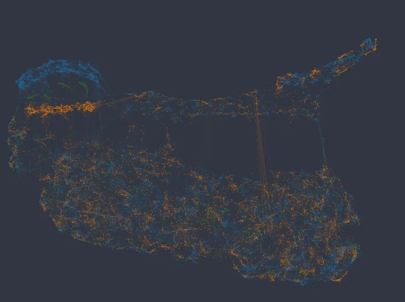
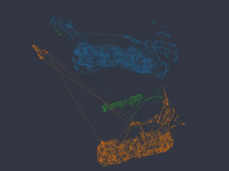
### k-NNG embedding
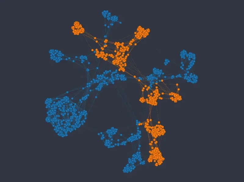
The k-NNG method produces the following layout:
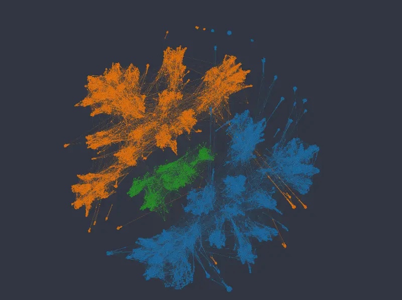
 Coloring in the top row by salary on the left, and department on the right, we see that the network forms clearly distinct clusters, and such that each cluster corresponds to a combination of the two kinds of categories. This is neither right nor wrong. And whether it's useful depends on the kinds of questions we're interested in. E.g. separating employees so clearly by department may or may not make sense in a specific scenario, since belonging to a specific department may or may not have a significance influence on other variables we may be interested in.
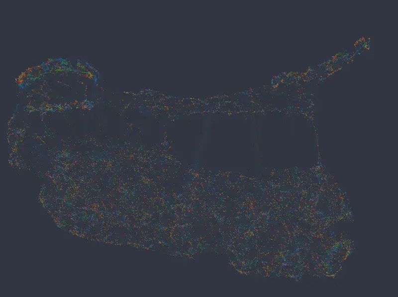
Within each cluster, points are organized according to the numeric variables, forming different directions/gradients of increasing or decreasing values etc. This is more visible in case of the ordinal-like variable *number of projects,* having 7 different values only, than in the case of *satisfaction level*.
### UMAP embedding
Using UMAP has the advantage of giving us more influence on the relative importance of categorical vs numeric variables. In Graphext, this can be done with the `type_weights` parameter, e.g.
```jsx theme={null}
embed_dataset(ds, {"type_weights": {"category": 4.0}}) -> (ds.embedding)
```
In the following series of figures we plot UMAP layouts with different weights being applied to categorical columns.
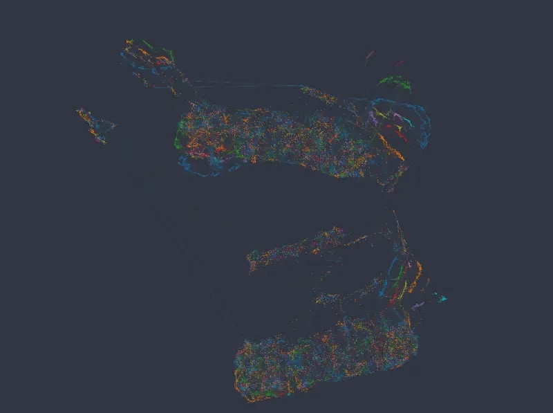
With default weighting, and using the same color mappings as before:
Coloring in the top row by salary on the left, and department on the right, we see that the network forms clearly distinct clusters, and such that each cluster corresponds to a combination of the two kinds of categories. This is neither right nor wrong. And whether it's useful depends on the kinds of questions we're interested in. E.g. separating employees so clearly by department may or may not make sense in a specific scenario, since belonging to a specific department may or may not have a significance influence on other variables we may be interested in.
Within each cluster, points are organized according to the numeric variables, forming different directions/gradients of increasing or decreasing values etc. This is more visible in case of the ordinal-like variable *number of projects,* having 7 different values only, than in the case of *satisfaction level*.
### UMAP embedding
Using UMAP has the advantage of giving us more influence on the relative importance of categorical vs numeric variables. In Graphext, this can be done with the `type_weights` parameter, e.g.
```jsx theme={null}
embed_dataset(ds, {"type_weights": {"category": 4.0}}) -> (ds.embedding)
```
In the following series of figures we plot UMAP layouts with different weights being applied to categorical columns.
With default weighting, and using the same color mappings as before:
 It is clear that UMAP in this case globally organizes the data according to similarity in the numeric columns, more so than according to the categorical columns.
Note, however, that *salary* data is not randomly or uniformly distributed here, even if that may seem to be the case at first glance. Even though the different levels of the categorical variables can be found spread across the entire network, they nevertheless tend to form little groups, i.e. nodes of the same category more often connect to each other than do nodes with different categories.
Increasing the weight of categorical columns to 6.0 (vs. the default of 1.0 for the rest), we see that data starts to separate into clusters representing different *salary* categories (top left e.g.).
It is clear that UMAP in this case globally organizes the data according to similarity in the numeric columns, more so than according to the categorical columns.
Note, however, that *salary* data is not randomly or uniformly distributed here, even if that may seem to be the case at first glance. Even though the different levels of the categorical variables can be found spread across the entire network, they nevertheless tend to form little groups, i.e. nodes of the same category more often connect to each other than do nodes with different categories.
Increasing the weight of categorical columns to 6.0 (vs. the default of 1.0 for the rest), we see that data starts to separate into clusters representing different *salary* categories (top left e.g.).
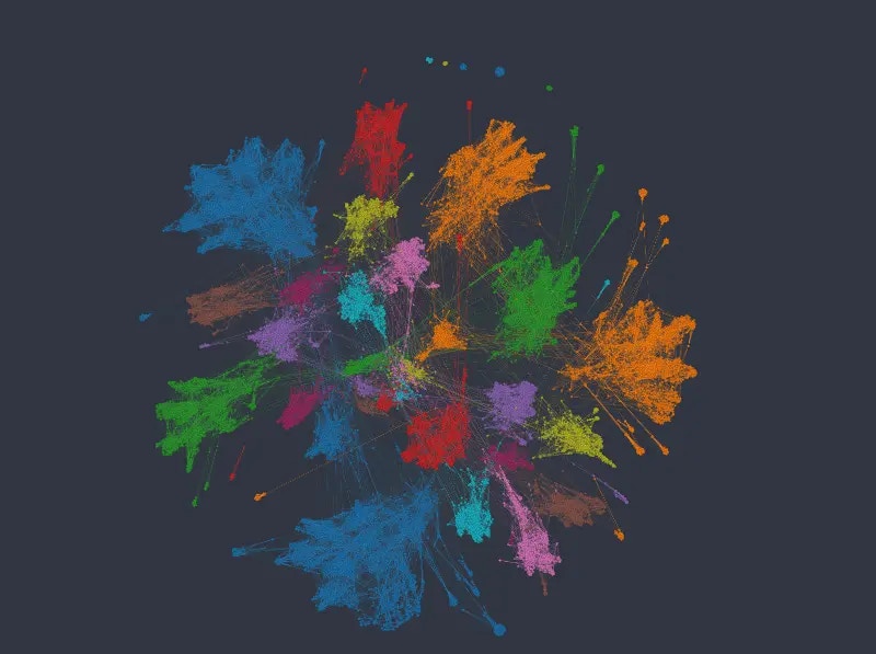
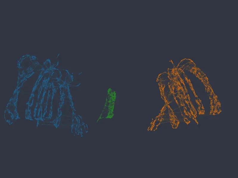
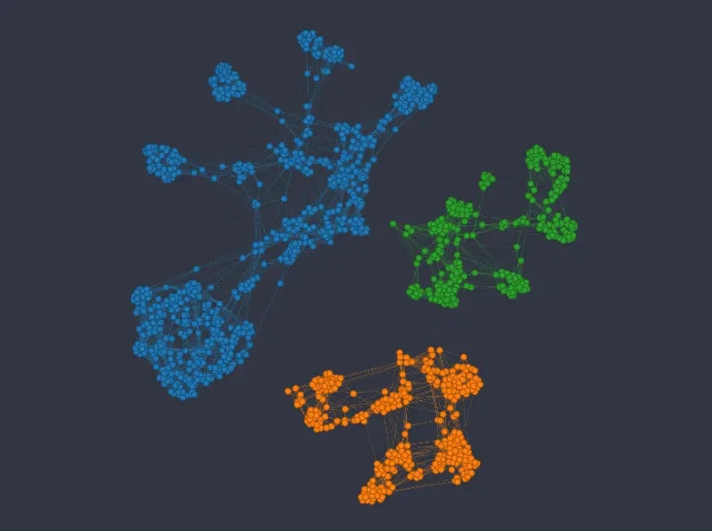
 With a weight of 8, the salary variable starts to dominate the global structure, and the network separates into 3 distinct clusters. The department variable also starts to separate parts of the network more clearly:
 The same tendency continues with a weight of 10.
 And with weights of 12 and 14 respectively, the network separates into completely distinct clusters, such that each cluster corresponds to a combination of the categories in the two categorical variables.
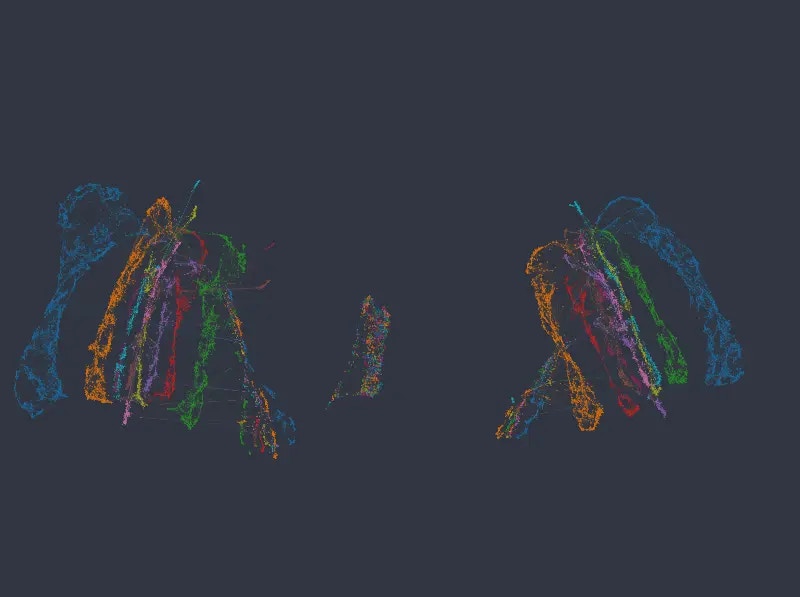
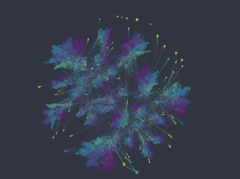
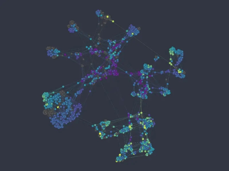
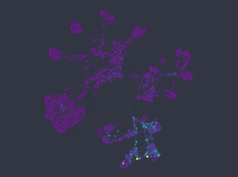
 Note that in no case are numeric columns ignored, even when the network separates into disconnected islands representing individual categories. The following figures again map color by our two numeric columns, using an embedding with categorical weight of 14:
 As can be seen, local structure in numeric variables is preserved inside and/or across the individual clusters. If anything, in a more organized manner than the original k-NN graph.
Note that apart from the above observations, UMAP also better maintains the relationship *between* clusters. While the relative positions of isolated clusters in the k-NN graph are completely arbitrary (as a direct implication of the underlying algorithm), UMAP is able to maintain the global structure inherent in the data.
## Example 2 – Titanic dataset
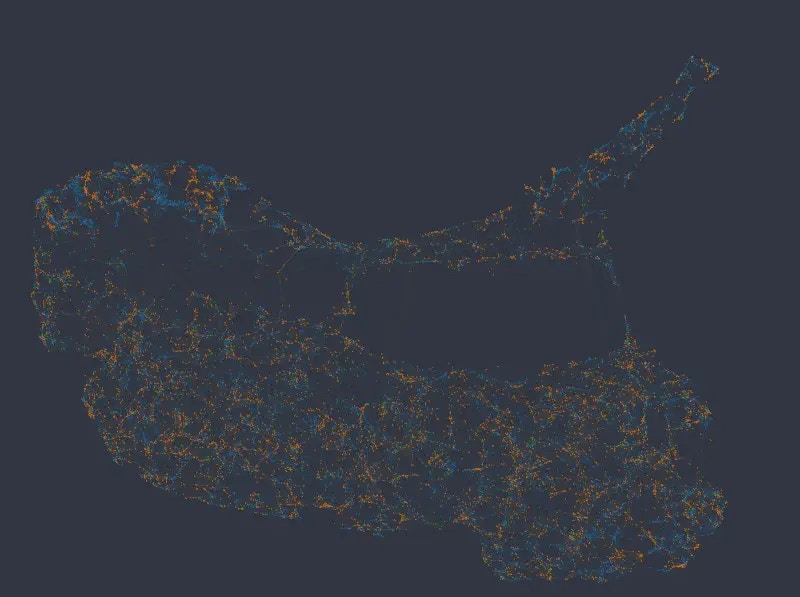
As a another example we will look at (a subset of) the Titanic dataset, which for each passenger contains 3 categorical columns (*sex*, *passenger class,* and *port of embarkment*), and 4 numeric columns (*age*, *number of siblings and spouses aboard*, *number of parents and children aboard*, and *fare price*).
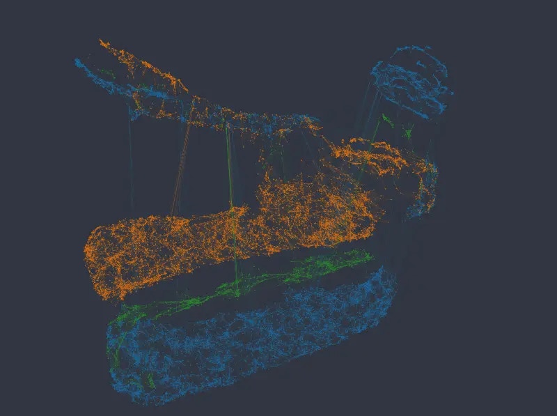
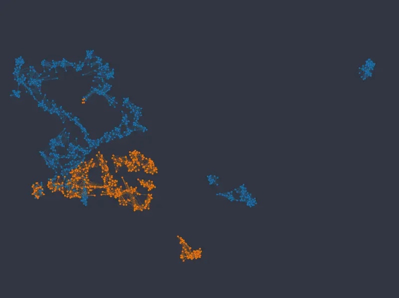
### k-NNG embedding
The k-NNG method produces the following layout (*double-click on an image to see a bigger version*):
As can be seen, local structure in numeric variables is preserved inside and/or across the individual clusters. If anything, in a more organized manner than the original k-NN graph.
Note that apart from the above observations, UMAP also better maintains the relationship *between* clusters. While the relative positions of isolated clusters in the k-NN graph are completely arbitrary (as a direct implication of the underlying algorithm), UMAP is able to maintain the global structure inherent in the data.
## Example 2 – Titanic dataset
As a another example we will look at (a subset of) the Titanic dataset, which for each passenger contains 3 categorical columns (*sex*, *passenger class,* and *port of embarkment*), and 4 numeric columns (*age*, *number of siblings and spouses aboard*, *number of parents and children aboard*, and *fare price*).
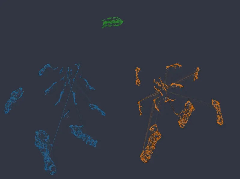
### k-NNG embedding
The k-NNG method produces the following layout (*double-click on an image to see a bigger version*):
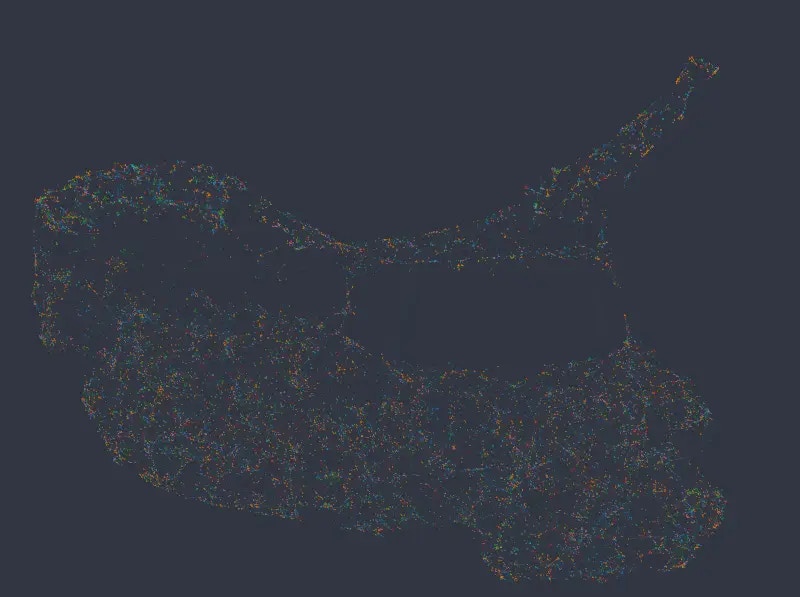
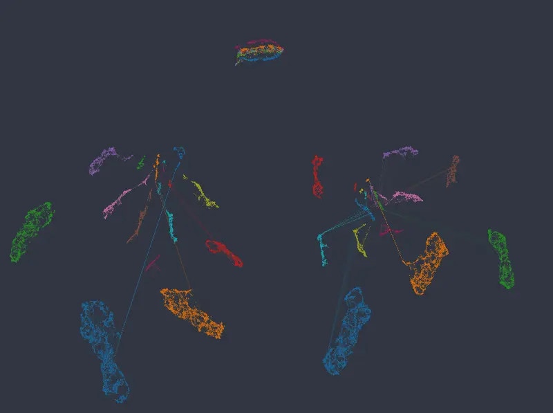
 As before we can see that the k-NNG method strongly separates different categories into separate clusters. Numeric variables than usually influence how nodes are distributed *inside* the clusters. Note that the approach seems to struggle somewhat in mapping the *age* variable\*.\*
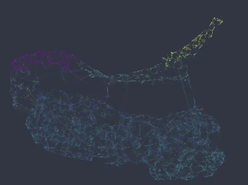
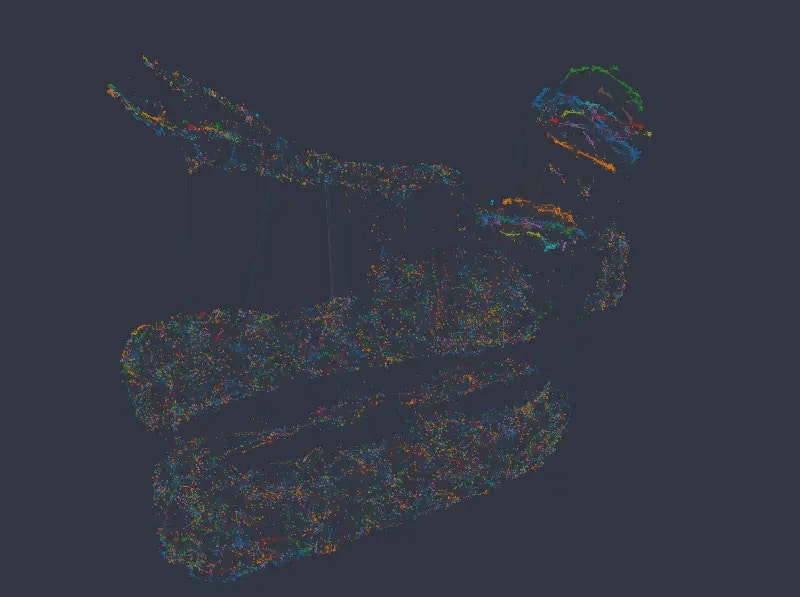
### UMAP embedding
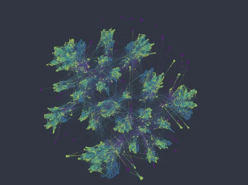
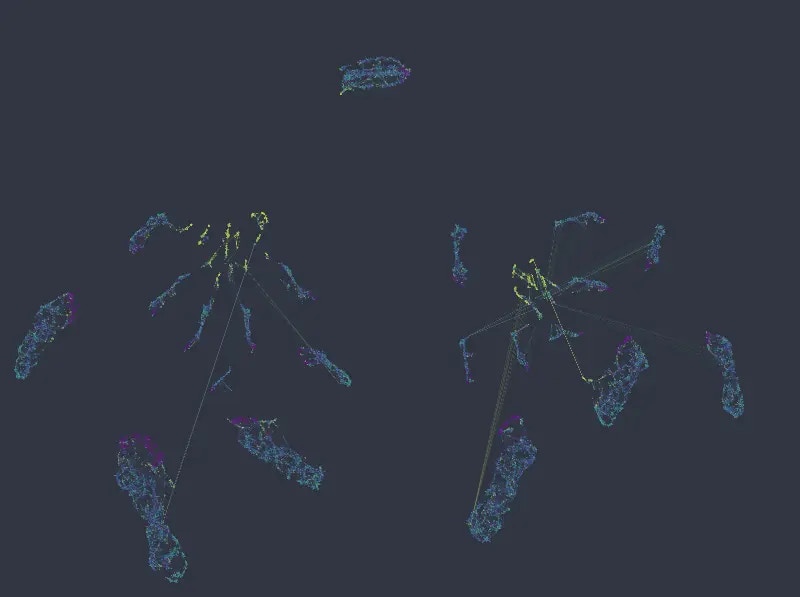
For this dataset, using UMAP with default column weights seems to achieve a good balance between categorical and numerical variables out of the box (note that in the following figures we changed the `min_dist`, and `n_epochs` parameters only, as with default values the resulting layout is rather thinly spread):
As before we can see that the k-NNG method strongly separates different categories into separate clusters. Numeric variables than usually influence how nodes are distributed *inside* the clusters. Note that the approach seems to struggle somewhat in mapping the *age* variable\*.\*
### UMAP embedding
For this dataset, using UMAP with default column weights seems to achieve a good balance between categorical and numerical variables out of the box (note that in the following figures we changed the `min_dist`, and `n_epochs` parameters only, as with default values the resulting layout is rather thinly spread):
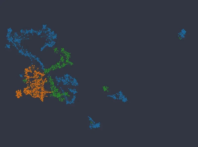
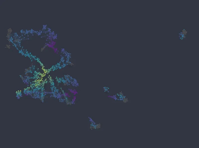
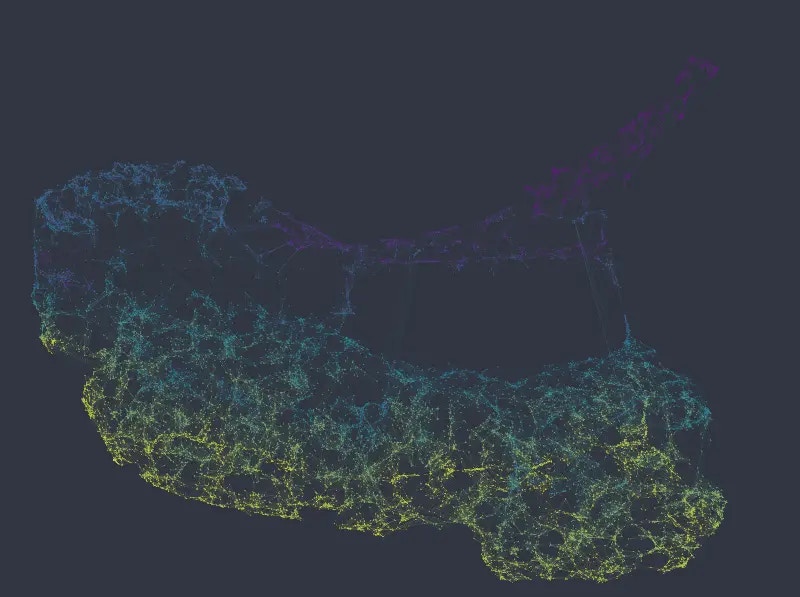
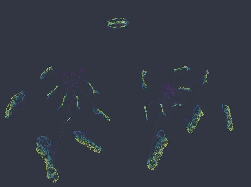
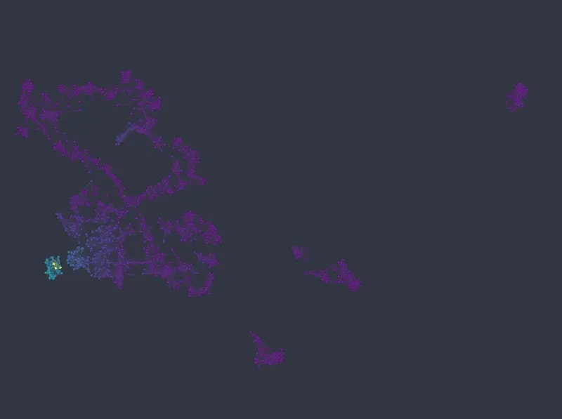 Note that not only are the different categories well represented by identifiable clusters, but numeric variables map much more cleanly to well defined areas or gradients in the layout, when compared with the k-NNG approach.
## Conclusions
As we have illustrated with two examples above, it is possible in many cases to tune UMAP embeddings such that the equilibrium between categorical and numerical variables corresponds to one's expectations (e.g. qualitatively matches results from the alternative k-NNG approach). Depending on the dataset, and the actual distribution of its data, the weighting required to achieve preferred results may differ. And so it is usually an iterative process to arrive at the final configuration. Also, note that not all undesirable layouts are due to the balance between different data types. Sometimes data may simply be distributed in such a way that no "clean" layout can be calculated that would still reflect the truth about the similarities of dataset rows. In other cases it may require tuning of UMAP's own parameters to achieve best results (see [Creating graphs and layout](/docs/recipes/graphs/create/) as well as Graphext's documention of the steps/methods involved, e.g. [embed\_dataset](/docs/steps/prepare/embed/embed_dataset/)).
Note that not only are the different categories well represented by identifiable clusters, but numeric variables map much more cleanly to well defined areas or gradients in the layout, when compared with the k-NNG approach.
## Conclusions
As we have illustrated with two examples above, it is possible in many cases to tune UMAP embeddings such that the equilibrium between categorical and numerical variables corresponds to one's expectations (e.g. qualitatively matches results from the alternative k-NNG approach). Depending on the dataset, and the actual distribution of its data, the weighting required to achieve preferred results may differ. And so it is usually an iterative process to arrive at the final configuration. Also, note that not all undesirable layouts are due to the balance between different data types. Sometimes data may simply be distributed in such a way that no "clean" layout can be calculated that would still reflect the truth about the similarities of dataset rows. In other cases it may require tuning of UMAP's own parameters to achieve best results (see [Creating graphs and layout](/docs/recipes/graphs/create/) as well as Graphext's documention of the steps/methods involved, e.g. [embed\_dataset](/docs/steps/prepare/embed/embed_dataset/)).